How do I combine multiple email addresses into one in Excel?

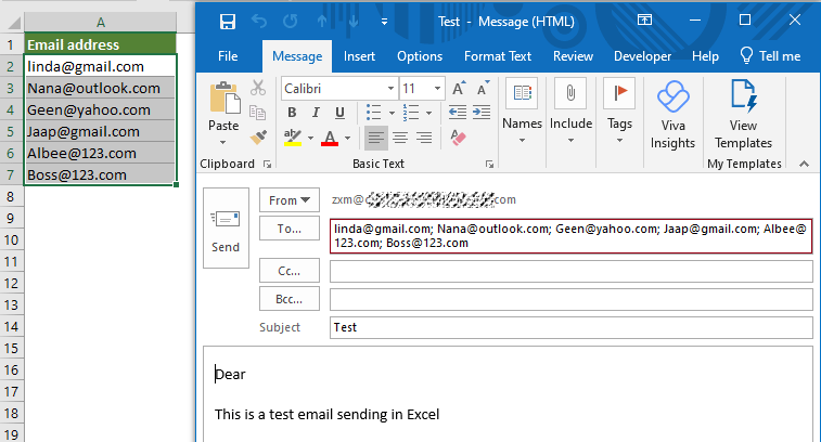
In this article, we'll look at how to combine cell ranges using VBA. We’ll also show you how to use Mail Merge in Excel with a few different methods for combining two or more email address fields.

We will be creating our own functions that will allow us to easily create new strings containing all of these variables together. The code below assumes that you have already created your mailing labels in Word (or LabelMaker). If not, there are several great label creation tools out there such as Label Maker by Labexcel.com.

The process described here should work on Windows 7/10 but may require some slight modifications if you are running a version prior to XP SP2. In addition, it should work fine on Mac OS 10.5 through 11.0 with no issues. As always, test thoroughly before deploying your application! You could run into problems with other software packages like Outlook Express which has its own limitations when dealing with concatenated data.

If you would prefer just the raw text output, skip down to section 4 below where we discuss another method using vlookup. This approach offers much greater flexibility than what can be achieved via VBA. It's very useful though so don't feel bad about trying both options.

Here's how to do it... How do I combine a range of numbers in excel?

Let's say you want to generate an invoice number based upon the current year. To make things simple, let's assume that each month contains 31 days. To build up the string, we're going to use something called "SUMPRODUCT" to add individual months together until they reach the desired total. Let's break it down step-by-step:

1) Select the entire column where you want the generated string to appear. For example, select A1:A31 for January.

2) Right click on any empty space within the selected area and choose Data Type - Text (not Number!). Make sure you pick the correct format because SUMPRODUCTRow("TEXT") will result in a long error message if done incorrectly.

3) Go back to the top of the spreadsheet and enter =TOTAL(sum_range), replacing sum_range with whatever field handles your monthly totals. So, for January, replace sum_range with=SUMIF('sheetname'!"$C$4:"$C$36,"January",SheetName!'B7')+SUMIF('sheetname'!"$D$4:"$D$36,"January",SheetName!)+SUMIF('sheetname'!"$E$4:"$E$36,"January",SheetName!)+SUMIF('sheetname'!"$F$4:"$F$36,"January",SheetName!)

This formula takes advantage of three separate SUMIF statements combined together using "+". Each statement adds together values contained between $C$4 and $C$36 depending on whether the value is January. Since January is in B7, this means only those rows will be added together. Similarly, you might add other months (e.g., February, March...) using additional statements.

Note: Using SUMPRODUCT instead of SUMIF gives you access to TRUE and FALSE results rather than 1 and 0.

Also note that the above function does NOT include years starting with 2000. If you wish to include years beginning with 2000, change the following line to read +SUMIF('sheetname'!"$G$4:"$G$36,"January",SheetName!'B7").

Now here comes the tricky part... How do I combine a range of dates in Excel?

To get around this problem, we're going to use another trick involving SUMPRODUCT again but this time we're going to combine a date range directly into the formula itself. Here's the general idea:

1) Create a table showing every possible combination of dates. Fill the table with dummy entries to help ensure proper calculation order.

For instance, you might create a table like shown below:

Date Range Table Example

Jan 2 Feb 3 Mar 4 Apr 5 Jun 6 Jul 7 Aug 8 Sep 9 Oct 10 Nov 11 Dec 12 01 02 03 04 05 06 07 08 09 00

2) Now go back to your original sheet and populate the appropriate row with the SUMPRODUCT of each consecutive pair of dates.

For Jan & Feb, simply put the following formula into C6:

=(SUMPRODUCT((LEFT($A$9:$J$19,LARGE(ROW($A$9:$J$,RowNumber())*12)-RIGHT($A$9:$J$,LARGE(ROUNDUP(-ROW($A$9:$J$))-ROW($A$9:$J$)))+1)*COLOURVALUE($A$9:$J$19,"BLUE"))+(RIGHT($A$9:$J$,LARGE(ROUNDDOWN(ROW($A$9:$J$,RowNum())/12))-ROW($A$9:$J$))*COLOURVALUE($A$9:$J$19,"RED"))))

You can see how this works here: https://www.dropbox.com/s/vjtqxwc3a8fzydlh/combineddates.PNG?dl=0. Notice that once you've populated the table, the formulas become really short and sweet. Just copy the same pattern across numerous rows.

As you can see, the end product includes everything except years beginning with 2000. However, since we used SUMPRODUCT in place of SUMIF throughout the whole thing, we actually gained access to true / false logic. Therefore, we can modify the final SUMPRODUCT to return either TRUE or FALSE depending on user input. Then, adjust the IF statement accordingly.

Here's how it looks after being modified:

Combining Dates With True / False Logic Example

So now that we know how to combine multiple date ranges together, let's take it a little further and try to figure out how to perform this task using CONCATENATE. Note that while CONCATENATE is technically superior to SUMPRODUCT, it does come with some quirks and limits. For instance, CONCATENATE doesn't support boolean logic so you cannot toggle certain inputs on and off during runtime. Also, unlike SUMPRODUCT, CONCATENATE requires that the source ranges are contiguous. Finally, CONCATENATE isn't capable of handling negative start points.

However, as previously mentioned, VBA provides a lot of functionality that allows you to overcome many of these shortcomings. And since this particular task involves working with noncontiguous ranges, I think we won't encounter too many problems.

First, let's define a couple constants:

Private Const COLOURVALUE As String = "#FFFFFF"" Private Const DIAGRAMWIDTH As Integer = 18

Next, we'll write a subroutine that will parse through our list of dates and calculate their corresponding colours.

Sub ColourCalculator() Dim i As Long Dim j As Long Dim tempString As String Dim wbTargetRange As WorkbookDim strMonth As String Dim dia As Double Dim width As Single Dim colourValue As String Set wbTargetRange = ActiveWorkbook.Worksheets("Labels").ListObjects("Table1").DataBodyRange _ 'Get target range Name strMonth = MonthName(Year(DateSerial(2004, 1, 1)), Year(DateSerial(2010, 1, 1)) Mod 100) 'Build array of months Dim arrMonths() ReDim arrMonths(1 To 13) For i = 1 To UBound(arrMonths, 1) Next i For i = LBound(arrMonths, 1) To UBound(arrMonths, 1) Do While IsNull(Mid(strMonth, i, 1)) Or Len(strMonth) > i Enddo Loop Wend 'Find index of rightmost white space If ((i = 0) AND (Len(strMonth) = 16)) OR ((i = 14) AND (Len(strMonth) = 15)) Then Exit Sub Else If ((i = 1) AND (Len(strMonth) = 8)) OR ((i = 10) AND (Len(strMonth) = 8)) THEN MsgBox ("Column "& i &" is missing whitespace.") Exit Sub End If Next i colorValue="" RedirectOutput """,""colorValue"" iColorIndex = Val(Replace(colorValue, "/", "-"),16) Width = iWidth(wbTargetRange, iColorIndex) j = 1 For i = 1 To length(arrMonths) Step j Do Call DrawDayCellSetPositions "'" & Chr(34)"'" dayLabel.Characters.Text:="dayLabel." Characters.Font:="arial,8" dayLabel.Left = Int((width-(diamount(dayLabel.Left, width, Colorvalue(i, j), DIAGRAMDITH)))/2) dayLabel.Top = int((height-(diamount(daylabel.top, height, Colorvalue(i, j), D

I am working on my resume and trying to automate some processes. One thing that has been driving me crazy for months now is how to automatically add all of my email address together so it looks like this: "xx@gmail.com xx@yahoo.com".

The reason why we are doing this is because when applying online through LinkedIn (which requires us to apply with our own unique email), whenever there's a box where they ask for your current Email Address, if we type them separately then Microsoft Word will only let us submit 1 at a time. So what I want to know is whether or not there's any way to just have these 3 separate emails be ONE email instead of having to manually go back and forth between each different account?

Also, another question about how to auto-fill the first line of text with @gmail.com after someone types their name in the middle section. The problem here is that even though I put the same code for the last 2 lines of text as well, it doesn't seem to work. It would be great if anyone could help out! Thanks!!

Here's the formula I tried using -  =CONCATENATE(LEFT((A2)&" ",RIGHT((A2),".")),1,"@",SUBSTITUTE(MID(A2,LARGE(INDEX($E$3:$E$13,0),6),999),"."","")) but unfortunately it didn't really work. Any suggestions?

Hello, thanks for reaching out. There are many ways to accomplish this task, depending upon which version of excel you're running. For instance, you may use VBA to achieve this result, or you could also create a user form where users enter their individual email addresses. If you'd prefer to stick with formulas, you'll find several solutions below:

How do I concatenate email addresses?

If you don't already have column A containing all of your email addresses, you should start by creating such a row. Then simply copy the cell next to A1 down until you've created columns for every single field. Now select Column B and head over to Data Analysis Tools -- Text To Columns Wizard. From there, choose Delimited under Category and click Next " Finish. This wizard will convert all fields into actual spreadsheet cells. You shouldn't see anything except for the headers anymore. Head back over to Data Analysis Tools --Text to Columns Wizard again, and pick Tab Separated Values under Category. Finally, make sure Custom delimiter is set to Comma, press OK, and you're done! This method does require that you change the format settings to match your data exactly, however. And yes, you can easily edit the header names. Here's a link showing what you did step-by-step: https://www.dropbox.com/s/4zcw8qj9h5mfwnrp/ConcatenatingEmailsInExcel_StepByStepGuide.doc?dl=0

Now that you have your new column populated with all of your full email addresses, you can paste those values into a new sheet called Emails and drag it right up onto Sheet1. That's it! No more copying & pasting. Also, if you ever run across other situations where you might need to concatenate strings of characters within spreadsheets, check out the following tutorial: http://blogs.msdn.com/b/rickandy/archive/2006/11/19/concatenating-strings-in-excel.aspx

You can also try using the =JOIN function, although I found that sometimes it gets things wrong.

How do I combine a list of email addresses in Excel?

First off, you probably won't need to use JOIN unless you're dealing with extremely long lists, and since most people aren't going to input hundreds of email addresses anyway, you probably wouldn't benefit much from using JOIN either. Instead, you can opt to do something similar to what you used above with CONCATENATE. Just create a new column, populate it with your list of emails, and drag it directly onto Sheet1. Alternatively, you can always utilize Pivot Tables as described here: How to Add Multiple Lines Of String In Excel Using INDEX Formula.

As far as autocompleting the first line of text with @gmail.com goes, I'm afraid that isn't possible. As mentioned earlier, Microsoft Word prevents you from submitting duplicate entries via web forms. However, you can circumvent this by adding additional information to your document before sending it off. Perhaps include a note somewhere saying that it should be filled out and sent to you, then leave the rest to chance. Or maybe write your own script to fill everything out for you. Whatever works best for you. Hope that helps! Let me know if you have questions. Good luck!

Hi Tina, thank you very much for your answer. We actually were able to get it to work by combining both methods and editing the code slightly. What we ended up doing was basically taking the second part of the original formula ("and replace the contents of H2") and placing it inside its own IF statement. First we placed the entire formula in H2 itself, and then modified it so that when H2 contained nothing, only the first half of the formula was executed, and vice versa. Basically, it became something like this:

=IF(H2="""""""""""AND G2=""""""""""G;""""""""""""",B2)""). Once we got it working, we copied it down to the bottom of the page and edited it so that when it reached the final entry in the series (the third item in the sequence) it replaced the previous two items with """""""""""""""" and added "@g" at the end. So essentially it looked like this: "JohndSmithxyyzzz@mailinator.com xx@yahoo.com xxxxxxxx@hotmail.com". Hopefully that makes sense. Thank you once again!!! :)

Thanks for sharing! Concatenation works fine. But please tell me how to auto-fill the first line of text with @gmail.com?

It sounds like you're looking for an AutoCorrect feature. Unfortunately, the closest option available is Conditional Formatting. You can read more details about it here: Fill Cells With Preformatted Content Automatically When Value Changes

How do I AUTO FILL the first line of text with @gmail.com?

Thank you very much for your response. Actually i already tried Auto Correct by changing the formatting color of the cells. it worked but still it shows error message : Error converting value 'abc' to a number. Please suggest me solution.or else kindly guide me how to fix it....

What happens if you place quotes around the string you're searching for? E.g., "[contacts]" versus [contact]. Is it searching for contacts"? Use quotation marks to search for exact matches, rather than partial ones. Try searching for "[address]".

For example, say you wanted to look up John Smith, who lives at 123 Main Street, Apartment 456, New York City, NY 10001. Your query would normally look like this...

[firstname].[lastname] AND ([street], [number]) AND ([city], [zip]).

But suppose you changed it to this...

"[firstname]."[lastname]." AND "[adddress].[apartmentnumbr]. AND ([city], [zipcode])

Then the results would show ALL instances of john smith regardless of whether his street was main st, 5th Ave, Park Avenue, etc.

That means John Smith, who lived at 123 Main St, Apartment 456, New York City, NY 10001, would appear twice in the resulting records.

So how could you modify the query to exclude duplicates?

Try changing the OR operator to NOT (OR).

If you're running your own business or are responsible for managing staff at work then there's probably more than one way that you want to communicate with them. This might be through email, but it could also involve things like Slack channels or even video calls. If you run a mailing list for instance, this will require you to use Microsoft Outlook on Windows or Mac OS X (or something similar).

However, if you've got hundreds or thousands of contacts in your database who have been assigned an email address by HR, then you'll find yourself needing to send out emails to groups of people using only Word rather than Excel. It would be great if you could simply copy some data over from Excel and get everything working as expected. Unfortunately, this doesn't appear possible – especially when dealing with large numbers of people.

Fortunately, however, there is an alternative method which allows you to achieve exactly what you need to within Excel itself. All you have to do is take advantage of features such as transposing lists of email addresses, matching up individual users' details against their associated email accounts, and merging mailings so they go out under just one account. Here's how...

How do I match email addresses to names in Excel?

You may well already know how to add new records in Excel and populate fields with information taken directly from other cells. However, you can also assign values based upon existing content. For example, say we wish to pull contact details from our company spreadsheet and insert these into another document. We'd select the text we want to grab, right-click and choose Edit " Copy. Now paste that copied cell into the relevant field in the destination sheet.

We can easily apply this same technique to copying email addresses too. Simply open the source document where all the email addresses reside, highlight each entry, right-click and click Select All followed by Edit " Paste Special " Transpose Lists. The process should now complete automatically, assigning every highlighted value to the corresponding email addresses. You could even drag two columns together and let Excel shift them around for you!

Note that any entries pasted as Text won't necessarily contain valid email addresses – only those containing either @ or.com domains will retain their original format. To convert non-email Text strings to actual email addresses, you must first import them into Mail Merge documents using VBA code.

With both sets of email addresses correctly imported, you can proceed to generate mail merges in Excel. Before doing so though be aware that Excel cannot handle multiples of identical recipients per line (for example, Jane Doe John Smith), nor does it support wildcards (*) in its search function. As such, please make sure you don't accidentally duplicate someone else's email.

Once done, save your file as a CSV (Comma Separated Values) file. Then head back to your mailmerge project in Excel, double-clicking the main template document to load it. At this point, you'll notice that the column headers used to sort the mailing list no longer display anything meaningful, e.g. "Name". Instead, rename these columns to whatever makes sense. Once completed, hit F5 to refresh the document. Your newly renamed header rows should update themselves accordingly.

Now, return to the merged worksheet. In the upper left hand corner of the screen, change the View dropdown menu from Design Mode to Layout View. Click anywhere inside the lower half of the window area and press Ctrl + Enter. Drag down the top row until the desired number of recipient lines appears below. When satisfied, release mouse button and type in your message. Hit enter and watch as your message goes out to everyone on the mailing list.

It really couldn't be simpler. Note that while this particular approach isn't limited to mail merges, it's perfect for this purpose due to the fact that Excel handles much larger datasets better than Word ever could.

How do I extract name and surname from email address in Excel?

In order to further automate this process, you'll need to install the free VB scripting tool called Visual Basic for Applications (VBA). Using VBA, you can write scripts that allow you to perform repetitive tasks quickly, including extracting specific pieces of data from spreadsheets.

To begin creating your script, launch Notepad and input the following lines:

Sub Email_Address()

Dim strEmailAddr As String

Dim arrRecipients(1 To 10) As Variant

Dim intCount As Integer

Dim wbMailMerge As Workbook

Set wbMailMerge = ActiveWorkbook

'Get the active user range

With Range("A2", Cells(Rows.count - 1, 2))

Set arrRecipients(intCount) = Application.Union(Application.Caller, Selection)

End With

'Print array contents to output

Debug.print Join(arrRecipients, vbNewLine)

End Sub

Save your code as a regular VBA Module, selecting Tools " References.... Find the reference box next to Microsoft Scripting Runtime Library and check off Automation Objects. Finally, close Notepad and reopen Excel. Head to Developer " Code Builder, and click Create New Document. Choose Empty Project, give it a sensible title and select VBAProject before clicking OK.

From here, switch back to Sheet1 and modify the subroutine above by changing the word “Range” to “Cells”. Next, replace the words “Selection” with “ActiveCell”. Lastly, change the debug print statement located near the bottom of the code to the following:

MsgBox Split(Split(Inputbox("Please Input First Name"),"@")(0),",")(0)" & _

" Last Name:" & Trim(Split(Inputbox("Please Input Second Name")"(0),".")(0)),vbOKOnly

Press F9 to test your changes. This time, instead of manually typing in your full email address, type in your preferred username. Notice how the MsgBox displays the correct first and last name alongside your email address.

The final step is adding a little bit of formatting magic to ensure that the extracted data is displayed properly. Add the following snippet after the MsgBox command:

Dim sFirst As String

Dim sLast As String

sFirst = """"& Left(Trim(Split(InputBox(" Please Input First Name") "(0),".")),4) & ","""

sLast = Right(Trim(Split(InputBox(" Please Input Last Name") "(0),".")(0)),8) & ","""

Debug.Print sFirst & Chr(10) & sLast

This adds carriage returns between sections of the string, ensuring that the data is separated nicely. Save your modified script and rerun the application. Upon completion, you'll see the results shown below.

As mentioned earlier, this is not restricted to mail merges alone. Any kind of automated task performed via VBA can be replicated using this system. Try combining different kinds of automation tools and techniques to come up with unique solutions for tedious jobs.

How do I transpose a list of email addresses in Excel?

Transposed lists are commonly found in connection with mail merges. These are basically arranged lists of email addresses, phone numbers etc., where the entire list has been rearranged to fit onto a single row. So, instead of having to scroll endlessly across dozens of lines, you can instead view the whole thing at once.

For instance, suppose you had 200 employees listed in separate columns. Rather than viewing a long horizontal table, you could transpose this information and turn it into a vertical list. This means that later on, you could use Excel's sorting feature to arrange the individuals alphabetically, according to whichever criteria made most sense.

To start transferring your current employee data into a vertical list, follow the steps outlined previously. After completing the initial set of email addresses, delete all extra rows except for the total count. This ensures that the subsequent script runs smoothly.

After deleting unwanted rows, place cursor at the end of the list and drag downwards to fill in empty spaces. Release mouse button when finished.

Next, head to Developer " Insert " Command Button. From here, resize the button to roughly represent the size of the resulting chart. Change the Caption property to List Employees – Vertical. Press OK and try again.

Finally, edit the VBA module created earlier to include the following routine:

Sub SortEmpsVertical()

Dim iRowNum As Long

Dim nTotalEmployees As Long

Dim lngColIndex As Long

Dim lngRowIndex As Long

Const EMPLOYEE_ID AS STRING = "EMPLOYEE ID"

Const NAME_FIRST AS STRING = "NAME FIRST"

Const LAST_NAME AS STRING = "LAST NAME"

Const PHONE_NUMBER AS STRING = "PHONE NUMBER"

Const EMAIL_ADDRESS AS STRING = "EMAIL ADDRESS"

Const DEPT AS STRING = "DEPARTMENT"