LIMITED SPOTS
All plans are 30% OFF for the first month! with the code WELCOME303
LIMITED SPOTS
All plans are 30% OFF for the first month! with the code WELCOME303

LIMITED SPOTS
All plans are 30% OFF for the first month! with the code WELCOME303

In previous versions of Microsoft Office, you could easily share entire spreadsheets by simply copying and pasting them into another document. But now, if you want to create a shared file that contains several different tables from various worksheets within one workbook, you can't just copy and paste those sheets as-is. Instead, you'll need to select which parts of each sheet are contained inside of this single document -- then save these selections as a "shared range." This is known as "sharing" and enables users who have access to this file to see multiple sheets at once without having to open up individual documents. Users will also be able to use formulas and functions across all of these selected ranges. To learn more about this process, read our guide below.
This article assumes you're using Excel 2010 (or newer) but most of the same principles apply to other versions too. We've included screenshots for both older and newer versions so you know what commands should look like regardless of when you last updated Office. If you aren't sure whether you're running version 10, check out our list of features added to Excel since 2000.
If you'd prefer not to follow along with this tutorial, you might consider creating a web app instead. Web apps let you embed any kind of content you wish, including spreadsheets, and they don't require installation on anyone else's machine beyond yours. You can even set permissions so people viewing this app won't necessarily have permission to make changes themselves. For more information on setting up a web app, take a look at our detailed guide here.
Note: In order to get the best results, we recommend saving files locally rather than over the network. That way, everyone has their own local copy rather than relying on someone else's server. If you must share via cloud services such as Skydrive, Dropbox, Google Drive etc., make sure to download copies first before opening them yourself!
The easiest method to accomplish this task involves selecting some data, right clicking, and choosing Copy [unformatted] Cells. Then, go back to where you want to place the copied selection, click the mouse button while holding down Shift key, and choose Paste Special... From the dropdown menu, choose Unformatted Values. Finally, head back to where you originally made the cut and paste, right click again, and choose Format Cells.... Under Category, pick Home Ribbon tab, then under Operations, pick Define Name... Enter a name for your selection, hit OK, and repeat until you cover everything you wish to keep track of.
Now, whenever you refer to the cell(s) that were just highlighted above, you'll start referring to the ones saved in the Shared Range field at the bottom left corner of the screen. The Shared Range field shows the location of the original source range and allows the user to view additional rows and columns after making the initial cut/paste. It looks something like this:
When finished, you may decide that you no longer need the copied cells anymore and delete the names you defined earlier. Deleting the name doesn't change anything about the underlying contents of the cell itself, however, because it was never actually stored anywhere outside of the Shared Range box. As long as you still have the actual values somewhere else, they'll remain unaffected.
For instance, if you had three separate worksheet tabs containing five rows worth of data, you would end up with 15 named cells total. When you delete them all later, none of the data stored inside of these cells will suddenly disappear. Instead, they'll continue working exactly as intended.
To show off more advanced techniques, try linking to a particular column instead of defining a whole row's worth of cut/pasted cells. Right click on whatever table you wish to link, select Insert Link to Cell..., type in the address of the desired cell, and press OK. A pop-up window will appear asking you to enter the exact reference number of the target cell. Type in column letter B2 for example, and press OK. After doing this, every time you write =B2+1&A7 in a cell elsewhere, it'll automatically update the value of the linked cell provided you used the correct syntax. Here's what my newly created link looked like:
As you can tell, this isn't quite as powerful as cutting/copying cells, but it does provide a cleaner solution if you plan to always display the same column throughout a given worksheet. Note that you cannot insert links between two nonadjacent columns, nor can you link directly to a formula. Also note that this command requires that your current cell contain text ("not numeric") otherwise it'll throw an error message.

Extracting columns from a large dataset often comes in handy when displaying subsets of data based upon criteria. Imagine you wanted to pull out all of the sales numbers for November 2011 from a massive.xlsb file filled with thousands of entries. Here's what you'd have to do manually:
Select the headers for all relevant columns
Copy and paste them onto a brand new sheet
Delete unnecessary columns
Sort the resulting table alphabetically
Once you've done this dozens of times for many different years, it becomes very tedious. Thankfully, there's a faster way to perform this action. Right click on the header row for the table, select Cut / Delete Row..., and choose Extract All Rows. Head back to your main sheet and select all of the data that needs extracting. Right click on the header and select Pasting Multiple Selection Rule... Choose Extracted Data Only and press OK. Your data will now be separated into smaller chunks according to its respective headers.
Here's what mine looked like afterwards:
You can also add further instructions to define custom rules depending on what you intend to do with each chunk. Make sure to preview your final result before hitting Finish though, especially if you're dealing with huge datasets that span multiple pages.
Sometimes you may wish to include tons of extraneous information in a spreadsheet that you definitely don't need elsewhere. Maybe you're sending this file to coworkers who use a completely different system that relies heavily on a lot of formatting info. Or maybe you're planning to email the file to someone whose computer runs Mac OS X. Whatever the case, sometimes you may only need to send a few columns consisting mainly of numbers. Fortunately, the previously mentioned technique of extracting rows can be modified slightly to achieve this goal.
Right click on the header row for the table, select Cut / Delete Row..., and choose Extract Last N Rows. Select all of the data you wish to extract, right click on the header, and select Pasting Multiple Selection Rule... Pick Columns Not Containing Numbers, and press OK.
Your data will now consist of only the columns specified in Step 2. Here's what mine looked like afterward:
Notice how the extracted rows weren't really deleted, despite being empty. They just became invisible because they fell beneath the threshold required to trigger the extraction rule. However, if you ever want to restore them, just highlight them individually and run through the steps listed above again to reinsert them.
Excel has always had one major drawback when using spreadsheets — you can't easily share parts of them. You could email someone a link to the document, but that would require them to have access to their own copy of Office and then open up Word (or whatever else) just to see what was going on.
Now, thanks primarily to improvements made by Microsoft over recent years as well as changes introduced in Office 2016, we're finally able to simplify this process considerably. We'll show you some of these methods below.
If you want to know more about the overall features available in Excel 2016, check out our guide here.
Previously, if you wanted to make any edits to certain data within a particular range of rows and columns, you'd need to send off the whole worksheet to whoever needed its contents. This is still possible through "copy-and-paste" instructions, but they aren't user-friendly at all. They also don't work very well, especially if you've got a large number of rows and/or columns involved.
The simplest way around this problem used to be to highlight the desired section, right click on it, select Properties, and then switch from Copy to Linked View. The resulting URL would contain the information necessary to display the highlighted selection properly without requiring anyone who clicked it to download anything. However, this method doesn't really cut down on clutter either. It simply moves the task of copying-and-pasting into other people's hands.
It does allow you to create links which will actually work even after months or years have passed since those links were created. But unless everyone who needs to view the sheet uses Internet Explorer 11, there are probably many users on older versions of Windows who won't realize that this option exists at all. Not only can the menus change depending upon whether you're running IE11, but so too can the properties themselves. In addition, most browsers nowadays automatically strip URLs like this from copied text anyway. So the end result isn't nearly as helpful as it should be.
A much better solution now seems to be to create two separate tabs containing different subsets of data within the same file. Then, whenever you want to edit something, you go directly to whichever tab contains the information you wish to modify instead of trying to manipulate a huge chunk of information every time. To accomplish this, follow these steps:
Select the row(s) and column(s) where the content lies. For example, maybe you want to update the first name field for all students currently enrolled in your class. Highlight the entire entry by clicking once above each cell in question until you get everything selected. Once this happens, press Alt+Down Arrow twice to move downwards past empty spaces while holding Shift to keep everything together. Right click anywhere along the top edge of your selection and choose Format Cells " Formulas... From the menu bar. If no such item appears, try selecting Insert " Formula Bar. That ought to put a formula icon next to the Ribbon's Home button. Clicking on it brings up the familiar =HERE() function. Finally, type "=" between the quotation marks and hit Enter. This creates a reference named "Student_Firstname", which refers back to the exact location where you chose to start highlighting earlier.
Click OK to exit out of the dialog box and continue onto step 2, where you'll repeat the procedure except that you'll replace the word Student throughout with the actual name of the student whose info you want changed. When you reach step 3, however, things might not look quite right because you haven't yet told Excel to refer to the current tab. To fix this, simply rename the tab via File --" Options--" General--" Tab Names dropdown list. Change the default label to whatever you called the original tab during Step 1.
Once you've done this, you'll notice that Excel automatically detects that the newly renamed tab contains the data you want edited. Just double click on the tab itself to activate editing mode, and you're good to go!
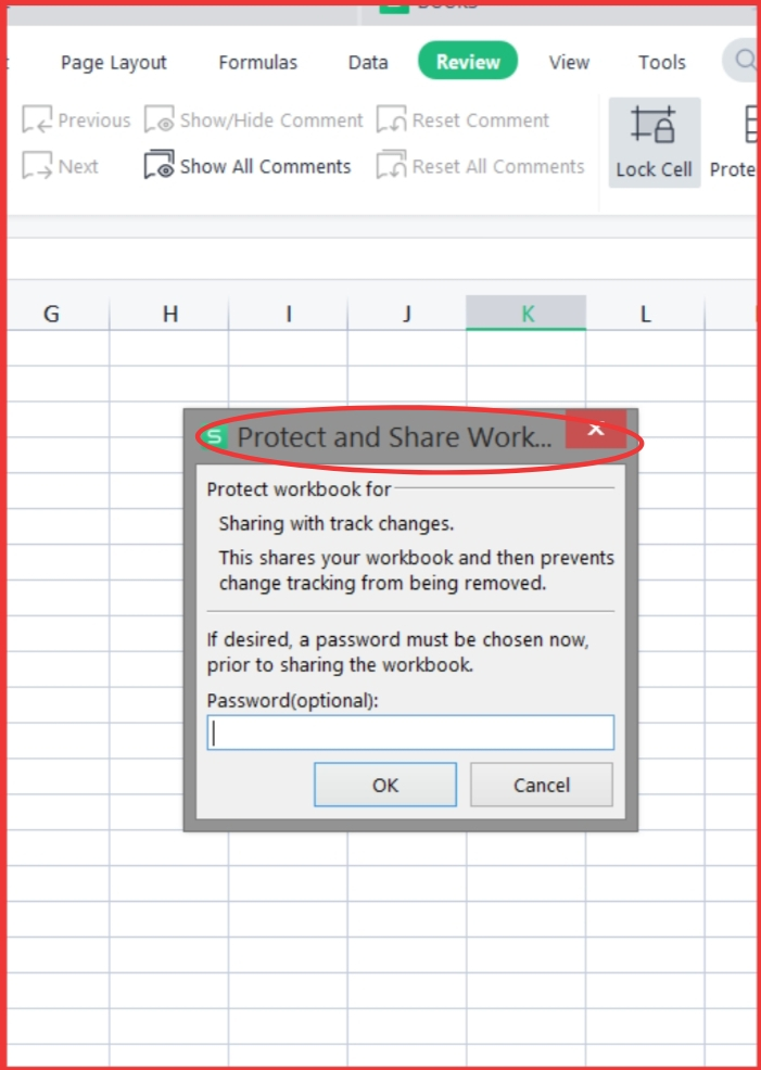
You can perform similar operations if you want to delete sections of data, although it's slightly trickier. Instead of renaming a tab, you must hide it altogether. First, navigate to File --" Info screen -" Protect Workbook... and set the value under User Interface Settings to No Protection. Next, head to File --" Save As.... Under Advanced save options, uncheck Create protected workbooks and give the file a unique name. Finally, return to File --" Information Screen --" Security settings and turn User Access Control Mode back to Protected View. This prevents further editing attempts by opening another person's version of the file.
This technique is useful mainly for deleting information. Unfortunately, if you're looking to completely remove existing data, you may find yourself unable to restore it later due to the aforementioned issue regarding linking formulas. Thus, it may be best to skip straight ahead to the section on exporting files below.
Before making any modifications whatsoever, let's take a moment to cover an easy workaround to avoid having to deal with the complications described above. Simply highlight the entire region containing the data you want shared. Then, right click on the left side of the selection and choose Quick Parts followed by Send to Web Page. A new window pops up asking for a web address. Type http://www.google.com into this space and press Return. After doing so, the highlighted data gets embedded as plaintext inside an HTML page hosted on Google's servers. Anyone viewing the page can then scroll through all of the data contained therein.
Unfortunately, the downside to this method is that the results are static. There's no real ability to customize or otherwise interact with the data in any meaningful way. Also, anyone wanting to add additional data to the mix will have to redo the whole process again.
But perhaps the biggest disadvantage to this approach is that it requires someone to visit Google's website just to read the data. Some people are perfectly happy keeping everything online, but others prefer to print hard copies of documents rather than accessing them through a computer monitor. And if you ever decide to rework the data or transfer it elsewhere, you'll need to contact Google directly and ask them to permanently host it on their servers. At least this way, you won't lose access to the data if you forget to renew your account.
In short, this method is fine for individuals who already use Google services frequently or who care less about customizing the output. Otherwise, it's kind of pointless.
As previously mentioned, this process involves creating multiple tabs and sending them to various destinations. Before getting started though, you'll need to determine exactly what you intend to achieve. Is it intended merely for personal consumption? Or, do you plan to publish it somewhere outside of your own home network? What sort of device will it run on? How big is the target audience? Will you include references to third party products or brands? All of these factors play a role in determining where you should upload the final product.
For instance, if you want to distribute the document publicly, then it's usually advisable to convert it to PDF format before uploading. Most modern computers can handle PDFs without difficulty, and they tend to retain formatting far better than normal XLSX files. Furthermore, converting it to PDF ensures that it remains usable regardless of operating system, browser, etc. Of course, if you're working locally solely to help someone else learn Excel, then feel free to stick with the native.xlsx format. Your recipients won't likely complain if you do.
To begin, simply go to File --" Export Selection... and pick one of three types: Normal ("All Sheets"), With Headers & Footer ("Sheet1"), or Without Headers & Footer ("Current Sheet"). Depending upon the purpose of your document, you may want to tweak this setting accordingly.
After picking this option, you'll be prompted to enter the destination folder path. Make sure to include the ".pdf" extension in case you didn't specify it manually. Hit Finish, wait awhile, and voilà! You now have a high quality digital copy of the chosen portion of your spreadsheet.
When dealing with columns of numbers, dates, percentages, currency values, etc., sometimes you may want to extract a single piece of data and pass it along to someone else. Perhaps you want to generate a report showing sales figures broken down per month. Or perhaps you're planning to compare prices across several stores. Whatever the reason, Excel makes it incredibly simple to grab a single column and deliver it wherever you please.
Simply locate the column you wish to isolate and drag it to the desktop. Go to Data --" Sort Area, and mark the checkbox next to Columns. Afterwards, click Manage Fields to pull up the Field Chooser dialog box. Here you can choose to either filter by Name or Index. Use the latter choice if you're interested in filtering by numeric position. Once you've picked your selection criteria, click OK to finish.
Excel is a fantastic tool that allows users to create spreadsheets from scratch or import them into their workbooks as.xls files. It also provides many useful features such as Pivot Tables and Charts so people can easily manipulate data within their spreadsheets. However, if someone else has access to those same spreadsheets then they could see parts of sensitive information contained therein. As a result, there are times when we need to restrict who can view our spreadsheets.
In previous versions of Microsoft Office (i.e., 2003 through 2007), restricting what other people saw was not very difficult but now things have changed. The latest version of Microsoft Office 2013 makes this process much simpler because users will be able to choose which specific ranges they want to hide. This means that by default all rows and columns will remain visible unless you go out of your way to change them. If you're using older versions of Excel then unfortunately hiding certain parts of your spreadsheets may require some more complicated methods. Here is how you can accomplish these tasks.
If you would like to keep certain parts of your spreadsheets hidden from prying eyes then you'll first need to decide exactly where you'd like to make adjustments. For instance, maybe you've created a list of names of employees and would rather keep their social security numbers hidden. By selecting "Data" at the top menu bar followed by "Protect Sheet," you can prevent anyone from viewing any cells containing either of these pieces of personal information.
To protect sheets individually, select File " Options " Protect Workbook.... Then check off the boxes next to Hide Rows and Columns and Hide Comments. When finished click OK and close the window. You should end up with something similar to the image below.
Now if you were trying to hide both sections of information then you must follow another set of instructions. First, right-click anywhere blank on your worksheet and select Format Cells... Next, under Protection Settings enter values for each option except Hidden Items. Selecting Hidden items will cause your entire spreadsheet to become fully protected.
Once again, click OK and close the window. You should get results very similar to the ones shown above. Note that even though you selected "Hidden Items" in step two, this does not mean that anything marked as hidden will still appear in your spreadsheet -- it simply ensures that all hidden elements will stay hidden. Also, remember that you cannot edit any of the settings after closing the window. So, once you finish making changes, save the document before closing the window.
Another important thing to note about protecting your spreadsheets is that once you apply protection settings they never revert back to normal until you manually remove them. Therefore, don't forget to take advantage of this functionality!
When working with large datasets it becomes necessary sometimes to extract portions of spreadsheets that contain too much information. In order to perform this task, head over to the Ribbon and navigate down to Home > Data Tools> Filter & Sort. Once inside this area, double-click on the column heading you wish to filter by and type whatever terms you would like to search for. Press Enter, and voilà -- every cell matching your criteria will automatically populate onto separate tabs.
You can copy and paste individual entries into different locations or delete unwanted records. To help ensure accuracy, try opening the original source file and copying/pasting the contents directly from that location instead.
Note: Be sure to always download copies of your filtered spreadsheets before deleting anything from them. Otherwise, you might accidentally erase valuable information.
One of the most common uses for Excel involves sending out reports via e-mail. Thankfully, if you know a particular section contains confidential information then you can send out a report without worrying about exposing everything. Simply highlight the range of cells you wish to include in your message and hit Ctrl + C. Head over to Word and open your document. Click Insert " Text Box " More Controls " Table " Horizontal Rules " Right. Finally, add text labels to mark each row and place them wherever you please. We suggest placing them near the bottom of your table in order to draw attention to them.
Click Done and insert your table. Make sure to add plenty of space between each label since you will likely receive responses asking why certain lines did not show up. Afterward, switch back to Excel and resize your selection box so that its height matches the size of your table. Hit Send E-Mail Message and you're good to go!
Yes, you can -- provided you know how to properly format the code. There are several ways to display content from multiple tabs simultaneously depending on whether you want to embed charts or images along with your tables. Here are two examples demonstrating how to obtain this desired outcome.
First example: Embed Images Using VBA Code
This method utilizes Visual Basic for Applications (VBA) programming language. Users will need to run macros whenever they want to update their documents' content. But here's the catch -- in order to execute commands within a macro users must press F5 while running your application.
Begin by creating a folder called MyMacros inside the root directory of your computer. Create an excel file called MacroTest.xlsm in this folder and open it. Within this file, you should find a subfolder named Macros. Double-click on this folder and select New Document. Give it a name such as DisplayChart1 and leave all options unchecked.
Next, head over to Developer " Events and double-click on Run_Command2. Choose Edit Command0 from the dropdown menu. A small black screen will pop up displaying the following line of codes: ActiveWindow.View.Seek SetActive = True Then Selection.FindWhat [---] FindText:=True Sub Test() Dim sht As Worksheet Dim rngCell As Range 'Dim strSearchString As String Dim intRowPosition As Integer Dim intColPosition As Integer Dim objIE As Object Dim lngIndex As Long Dim intCount As Integer i = 0 While 1 i = 2 i = 4 i = 6 i = 8 End While With Sheets("Sheet3").Activate.Range("A7", ("[--]")) Do While Len(Trim((objIE.Document).getElementById("""").innerHTML "")) And Not IsEmpty(Split(Trim((objIE.Document).getElementsByTagName("table")(0).rows "(-""), "["])(0)), "(") ) Do If Trim((objIE.Document).GetElementsByClassName("cell"(0)).Item(0).childNodes "(-"").Value) Like "*dummy*" Then MsgBox (.Address(0) & ", Cell number: " & Int16(i / 3 * 7) & ", Row: " & i) Exit End If Loop Until ((intRowPosition - 5) Mod 6) = 0 i = (i + 1) / 3 End While objIE.document.parentWindow.[http://www.w3schools.com/htmlref/metatile.asp?oid=MTAuMTBodBC]SetAtr([http://www.w3schools.com/htmlref/ts_textbox.asp?name=TSAttribute_OnChange&value=[http://www.w3fools.com/?code=%26txt%3D%253Cscript+type+%255Bvar+myVar+%257Bbreak++%253Boutput%2521])][https://www.google.co.uk/search?hl=en&client=firefox-a&q=site%20url+encoded+input+onchange&btnG=Google Search&aq=f&oq=site%20url encoded input onchange])End With End Sub Go ahead and press F5 to launch your program. Notice that nothing happens immediately; however, if you wait five seconds you will finally see the results displayed in the command prompt window.
Second Example: Use ChartObject Properties Instead Of VBA Codes
The second approach displays embedded objects such as charts and graphs in addition to tables. This method requires no coding whatsoever. All users will need to do is activate the chart and drag it across the page. Begin by adding three empty charts to your spreadsheet. Each chart should consist of four series -- namely Series 1, Series 2, Series 3, and Series 4.
Head over to the upper left corner of your workspace and select Insert " Illustrations " ChartObject. Pick whichever chart you wish to utilize and rename it appropriately. Next, double-clicking on the new object will bring up the properties panel. Switch over to the Axis tab and scroll down until you come across the CategoryNames property. Change this value to match the titles of your series. Repeat this action for all of your axis labels.
 Send emails at scale